
Patient Satisfaction Dissertation
December 25, 2020
Investigating the Impact of Sustainable Solar Energy Development in the Kingdom of Saudi Arabia
December 30, 2020
Designing Model Predictive Control for the Shell Control Problem involves creating smart strategies to manage processes efficiently. It's like teaching a computer to make smart decisions to keep things running smoothly at Shell. Creating a Model Predictive Control system for Shell's control issue involves designing a smart solution to manage their processes efficiently.
Executive Summary
This section of the paper will present a comprehensive summary of the subject under study, presenting detailed information on the Model Predictive Control System, Shell Control Problem, the control system's design and the relevant parameters of the subject of study.
Chapter: Literature Review
Incorporating an automated control strategy for anticipating and/or predicting into any process system is logical and systematic; hence, Model Predictive Control (MPC) has undergone notable development in the course of the past twenty years, both inside the industry and in the research control group. Predictive control can be described as an approach rather than a specific algorithm, as its utilization is based upon interpreting an approach to define the algorithm that best suits the user requirements.
Discover the Significance of BIM in Design Coordination
Prediction provides pivotal information on how the system is expected to respond when exposed to certain conditions. Humans have a natural prediction and response system which supports our day-to-day requirements, and in some way, PID can be deconstructed as a derivation of human technique for obtaining control of simple systems. A predictive control incorporates measurement and decisions made on the measurement via introducing the feedback loop. Therefore, a model is required to automate predictions by measuring the available data.
For example, a driver anticipates future demands, targets, distances, speeds of other vehicles/pedestrians, etc. Therefore, the driver anticipates/predicts, and responds with effective control strategies in accordance with the given/assessed data to drive safely. This effective prediction provides us with the most desirable future outcome and thus seems logical. This logical concept can, therefore, be developed into automated strategies incorporating constraints explicitly enabling optimum constrained performances.
Model Predictive Control is the most general method for representing the process control problem in the time-space. The primary concepts of the MPC are;
- Prediction
- Receding Horizon
- Modelling
- Performance Index
- Degree of freedom
- Constrain handling
- Multivariable
The integration and/or derivation of these primary components allows stochastic control, optimal control, multivariable control, dead time procedures control and references in the future. Due to its use of the finite control horizon, MPC offers another advantage of handling constraints and non-linear processes in general.
Although MPC is indeed considered to provide robust control in most common applications, proofs regarding its robustness and stability have been hard to collect due to its utilization of the finite horizon. This has proved to be a disadvantage for a more extensive spread of MPC within the control research group. There are some new results which are very promising about the expansion of MPC within this community in a brief period. On the contrary, although various applications have been accounted for in industry and research centres, MPC has not yet achieved its expected industrial application, as it is still being developed for complex dynamic processes. One explanation behind this is that its usage obliges some numerical complexities, which are not an issue for the research control group but are a disadvantage with respect to the utilization of the technique by control engineers during practice.
The term Model Predictive Control does not assign a particular control method but rather a sufficient scope of control strategies which make express utilization of the process model to acquire the control signal by reducing an objective function. As a result of these design methods, controllers are obtained with basically identical structures and present satisfactory degrees of freedom. The ideas which show up in greater or lesser degree in the predictive control family are essentially:
- Explicit mode utilization to anticipate the output of the process at a time in the future (horizon)
- Estimation of a control arrangement to minimize an objective function and
- Receding strategy, which ensures that at every moment, the horizon is displaced in the future
The different MPC calculations (e.g. Receding Horizon Predictive Control (RHPC)) vary from each other in the model used for process representation and minimization of noise and cost. This sort of control is open, in which numerous works have been produced and are generally welcomed by the industry and the academic world.
Numerous successful predictive control applications exist, which are not only confined to the process industry, as their various applications to control different mechanical/other processes have succeeded in recent decades. These include robotic engineering (Ortega and Camacho, 1996), clinical anaesthesia (Linkers and Mahfonf, 1994) and many others. Its utilization in cement manufacturing, robot arms and drying towers are discussed in detail by Clarke in 1988, whereas potential improvements in the PVC plants, distillation columns, servos or steam generators have been outlined in the research conducted by Richalet in 1993.
The great execution that these applications display demonstrates the potential of the MPC to accomplish exceedingly effective control systems designed to work for long-time durations with barely any intervention required.
MPC offers a variety of advantages over the rest of the available methods, the most important of which are as follows:
- The staff with limited control awareness is particularly attracted to this methodology since the ideas are mainly intuitive, and the tuning is moderately simple.
- It can control a wide range of processes, from those with moderately straightforward structures to more complex systems, incorporating those with long delays continuing and or altering operational phase requirements.
- It is easy to deal with the multi-variable case.
- Feed-forward control is presented naturally to make up for measurable disturbances.
- It naturally recompenses for dead times.
- Its augmentation to treat constraints is reasonably straightforward, and these might be systematically included amid the design phase.
- The product is a controller, which is a simple-to-execute control law.
In spite of the fact that the application/utilization of control law is not difficult to implement and does not require performing many complex calculations, its formulation is more intricate than that of the conventional PID controllers. In the event that the process dynamic has no change, the formulation of the controller is possible in advance, but in the case of the adaptive control, all the calculations must be completed at each testing time.
At the point when constraints are incorporated, the measure of processing needed is significantly higher. Despite the fact that this is not a key issue (considering the computing power available nowadays), it should always be under consideration that numerous industrial process control workstations are not in their perfect form of computing, data, and most importantly, that the majority of the accessible time at the process workstation must be utilized for tasks other than calculation on the control algorithm itself (recording, communication, alerts, and so on). Indeed, along these lines, the biggest disadvantage is the requirement for a proper model of the process to be accessible. Prior model knowledge is the base for the design algorithm, yet the acquired benefits will be influenced by the differences existing between the real process and the model.
In the industry, MPC has established itself as a sensible methodology for industrial control despite the initial absence of theoretical results at some pivotal issues, such as robustness and stability.


MPC Strategy
To define the strategy of MPC, it is first important to highlight some of the basics of MPC modelling. The simplest model to develop to provide accurate enough predictions is considered to be the best possible model, as excessive effort in improving the accuracy of the model may complicate the model with very little enhancement in efficiency. The MPC steady state simple models have objectively produced up to 80-100% accurate predictions that capture key dynamic changes during transients. It is also important to note that the feedback’ normally corrects itself for small modelling errors.
The performance index can be defined as the accuracy to which the input trajectory behaves for a process in the automated predictive control strategy. The performance index is also designed to follow a simple set of conditions to obtain simple optimization. However, for complex systems requiring more control and precision measures, the performance index design becomes more demanding. High performance implies risk regarding the ability to deal with uncertainty or robustness. The degree of freedom, which is defined as the complexity of input predictions, behaves in the same pattern as the performance index. The useful number of degrees of freedom is associated with prediction accuracy, and varying set points or targets in a system requires more degrees of freedom. The simpler analogy is to define a model with a polynomial of first order, with data fit in a small domain. With a low prediction horizon, it is impossible to compressively anticipate a process's outcomes, which may lead to an ill-posed problem.
The predictive control can systematically embed constraints into the strategy development, which is critical for obtaining effective and robust closed-loop behaviours. Embedding constraints, such as water flow in process control, ensures that the integrated input strategies are optimized according to the operation set point and desired tuning requirements, incorporating a much more effective design than a standard PI control.
All the controllers of the MPC family utilize the methodology which can be characterized by the following strategy, represented in the figure given below;
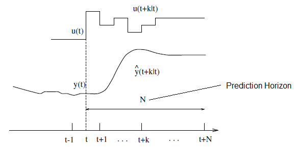
The process model can be used to predict/anticipate the future values for a resolute horizon N (prediction-horizon) at each instant. This anticipated output values y (t+k | t) 1 for k equals to1 to N, depending upon the determined/known values up to the time t (past outputs and inputs) and also on the control signals in the future u (t+k | t), where k is between 0 and 1 less than N, which are the input values given/fed into the system of the simulator to be calculated
By keeping the designed process closer to the reference trajectory w (t + k) through a determined criterion, the future control signal set is computed, which might be the set point itself or a close estimation. This determined criterion is usually in the form of a quadratic function, which outputs the error values between the predicted reference trajectory and the predicted output signal. The objective function incorporates the control effort under most circumstances. Given that there are no constraints, an explicit result can be calculated if the model is linear and the criterion is quadratic; otherwise, there is a need to use an iterative optimization method.
The process receives the control signal u(t | t) while the control signals being received after this time t are rejected because at the next sampling time, y (t + 1) is known in advance, and step 1 is now performed again with this new value, followed by the update of all the sequences. Hence, the value of u (t + 1 | t + 1) is processed, which on a fundamental level will not be the same as the u(t + 1 | t) due to the new data access, utilizing the concept of receding horizon.
The basic structure of MPC can be demonstrated in the figure presented below;
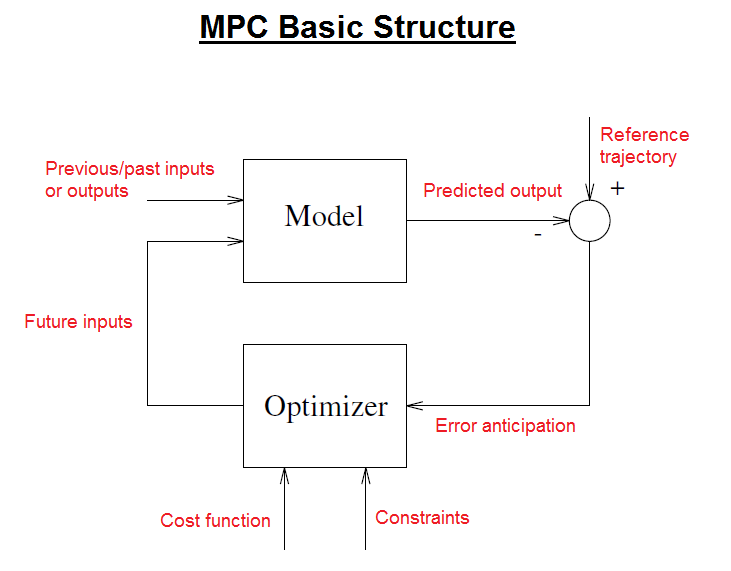
The model is utilized to foresee the future outputs of the process/plant, depending on the past and current values and on the proposed ideal future control activities. This optimization evaluates these activities considering the cost function, where the future tracking error is taken into account, and all the constraints. Hence, the role of the process model in the controller is decisive. The selected model must be able to capture the process dynamics to accurately predict future values and be easy to understand and implement. Since MPC is not a single method but rather a set of distinctive techniques, there can be numerous sorts of models which can effectively be utilized in different situations and conditions. The selection and design of the model are based on the user requirements.
The Truncated Impulse Response Model stands out among the most prevalent techniques currently used in the industry. This model is extremely easy to understand, as it just requires calculating the output when an impulse input excites the process. It is broadly acknowledged in industrial practice on the grounds that it is exceptionally intuitive and can likewise be utilized for multivariable processes, in spite of the fact that its primary disadvantages are the vast number of parameters required by it and only the open-loop stable processes might be modelled along these lines. A similar model is the Step Response Model, derived when there is a step input.
Perhaps the State Space Model is more common in the academic research group due to the simplicity of its derivation, even for the multi-variable case. The state space description makes the robustness criteria and the stability expression much simpler. Academic researchers additionally utilize the Transfer Function Model, and even though the controller derivation is more complex, it needs fewer parameters. It can handle dead time with much more ease compared to other models. Compared to state space, this model type is better understood in the industry because a portion of the concepts utilized by its transfer function, for example, gains, time constants and dead time, are generally utilized in industry. This description is common, to some degree, to both industry and academia.
Explore Key Innovation Management Models
Another major part of the MPC technique is the optimizer, which is the source of the control actions. In the event that a quadratic expression is obtained for the cost function, its minimum might be formulated as a linear function of past outputs, inputs and the future reference trajectory. In case of constraints such as inequality, the result must be calculated through the numerical algorithms, which require more computations/simulations. The optimization problem complexity relies upon the number of variables and the prediction horizons utilized. It generally ends up being a modest optimization problem which does not oblige complex computer codes to be solved.
It is important to note that the measure of time required for the robust and constrained cases might be many times larger than the required for the unconstrained case, and the processing bandwidth to which constrained MPC could be applied is considerably minimized.
Perceive that the MPC procedure is fundamentally the same as the control system utilized when driving a car. The driver is aware of the coveted/perceived reference trajectory for a finite control horizon and by considering the car's attributes. The driver selects/chooses one of the many control activities, such as brakes, accelerator, and steering, to follow the desired trajectory. Just the basic control actions are performed at every moment, and the method is repeated for the following control choice in a receding horizon style.
Recognize that when utilizing traditional control techniques, for example, PIDs, the past errors are the base for future control actions. The analogy of driving a car, which was used in an example earlier in this literature review, has also been carried out by one of the MPC vendors/designers known as SCAP (Martin and Rodellar, 1996), which states that the PID method for driving the car would be identical to driving it simply utilizing the mirror. This relationship is not completely reasonable with PIDs because MPC utilizes more data (the reference trajectory). Recognize that if a future point in the reference trajectory that is desired has been utilized as the set-point for the PID, the contrasts between both control methods would not appear to be so abnormal.
The following section centres around predictive control technologies that have a considerable effect on the industry and are accessible in the commercial sector, also considering different topics such as short application summaries and the constraints of the current technology. Despite the fact that there are organisations that limit the innovations created by them to their usage only, the following companies might be viewed as illustrative of the current technology development of Model Predictive Control. Some of the names and acronyms of their products are Adersa’s Hierarchical Constraint Control (HIECON) and Predictive Functional Control (PFC), AspenTech’s Dynamic Matrix Control (DMC), ABB’s 3d-MPC, Treiber Control’s Optimum Predictive Control (OPC) and many more. It must be noted that every product is not just the algorithm but includes extra packages, normally plant tests or identification packages.
A huge number of MPC applications are currently being applied in various industries. Qin and Badgwell previously reviewed these applications in the late 20th century. The petrochemical and chemical refining industry has been one of the oldest users of various application fields of MPC, as it enjoys a strong foundation in this field. Other considerable development territories incorporate pulp and paper, aerospace, food processing, and automotive enterprises. Different zones, for example, furnaces, gas, mining, utility, or mining, likewise show up in the report.
A few applications in the cement business or pulp production lines, especially in the United Kingdom, have been discussed in detail by the research conducted in 1996 by Martin and Rodellar. In spite of the fact that MPC innovation has not yet profoundly established its usage in territories with strong process non-linearities and frequent operational condition changes, the amount of non-linear MPC applications is now considered to be increasing.
Research completed by Muske and Rawlings (1993) indicated that there are various limitations of the MPC technology when employed in the dynamics processes of industries. As highlighted in this research, the most significant limitations include the over-parameterized models, as most of the commercial methods utilize the plant's impulse or step response model, which is known to be over-parameterized. For example, a transfer function might modulate a first-order process utilizing three parameters (time constant, gain) to depict the same dynamics. Moreover, these models cannot be employed for unstable processes. These issues could be overcome through the use of an auto-regressive parametric model.
The tuning process is another parameter that is not well characterized since the trade-off between closed-loop behaviours and tuning parameters is often unclear. In the presence of constraints, tuning may considerably be more troublesome, and it is not simple to ensure closed-loop stability, even for nominal cases. This is the reason why so much exertion must be directed towards prior simulations. The problem feasibility is one of the most difficult areas of MPC; therefore, much of the research is being conducted in this field of study.
Dynamic optimization suboptimality: many packages offer suboptimal solutions to minimize the cost function with a specific end goal to accelerate the time for results. It could be acknowledged in rapid applications (tracking systems), where tackling the issue at each sampling time may not be possible. However, it is hard to support process control applications unless it is demonstrated that the suboptimal result is constantly practically optimal.
Despite the fact that model identification packages provide assessments of model uncertainty, only one of these packages (RMPCT) utilizes this data within the control design. The rest of the controllers might be tuned again to enhance robustness, even though the connection between robustness and performance is still unclear. A sensible supposition would be to consider that the output disturbance will stay steady in the future; better feedback would be conceivable if the disturbance could be measured more precisely.
An efficient investigation of MPC's robustness and stability properties is impractical in its original finite horizon formulation. The control law is mostly time-varying and cannot be represented in the standard closed-loop form, particularly when constraints exist. Moreover, the results acquired by the researchers about robustness and stability are limited to small-scale processes (limited control horizons and state space) only.
Engineering is consistently advancing, and the new technology will need to face new difficulties in open topics, for example, identification of models, unmeasured disturbance forecast and estimation, modelling error treatment, and nonlinear model predictive control uncertainty. Despite critical progression in control algorithms and process control hardware, most process control problems nowadays are handled through sequencing, logic and PID controllers. There are, however, a few indications of change. Dynamic matrix control and similar algorithms are utilized on a couple of hundred frameworks, typically in supervisory loops with essential control still with PID controllers. Primary control loops have also started to be affected by advanced control. It can be roughly approximated that in excess of 100,000 loops use adaptation and automatic tuning. Despite 100,000 being a large number, this is still just a small portion of the total quantity of industrial feedback loops.
The drivers behind this development are the advances in computer technology and information infrastructure, client requests, control theory and challenging problems. Recent announcements by the makers are great evidence that the innovations have a huge effect.
In 1986, the Shell Company first published their benchmark control problem in the First Shell Process Control Workshop (Prett and Morari, 1987). It gave a realistic and standard testing ground for assessing new control theories and techniques.
Shell's heavy oil fractionator process is multi-variable and has many constraints, with large dead times and strong interactions. The Shell benchmark control problem is undoubtedly complex and needs efficient algorithms and control architectures to perform its desired control outputs.
Receding-horizon control (RHC), model predictive control (MPC), or moving-horizon control (MHC) is a prominent method that has been effectively utilized as a part of the control of different linear and non-linear dynamic frameworks. Shell developed the quadratic dynamic matrix control algorithm (QDMC) for their Shell benchmark control problem. The principal advantage of QDMC is that the constraints and targets connected with the control problem are implanted into the control algorithm, which needs small and hoc controller modifications. However, the downside of QDMC is its computational needs are intensive, bringing about the need for online computation. This is the fundamental detriment of MPC and limits its use to moderately quick and/or vast processes with a larger number of inputs (Clark and Mohtadi, 1987; Richalet, 1993).
In reality, there are many complex high-dimensional frameworks in which the amount of constraints and variables is often as large as a few hundred. Hence, it has become extremely critical to create computationally efficient control algorithms and architectures with less burden of computations. Unfortunately, there are few references for this topic in open literature; however, influential research has been conducted in the last many decades, such as by Ricker and Lee, 1995 Xu, Xi, and Zhang, 1988; Zheng and Allgower, 1998; Katebi and Johnson, 1997, Van Antwerp and Braatz, 2000, and Zheng, 1999; to demonstrate the large scale nature of average industrial plants. This is most likely attributable to the natural troubles in the complex computation for this large framework.
With the rapid and continuous advancement of communication systems and field-based engineering, control that is central has not been an essential characteristic in applications, and it is being slowly substituted by distributed control in large-scale frameworks. Distributed control structure brings new prerequisites to the conventional control field and provides an opportunity to solve new difficult control applications. To accommodate monetary issues and avoid degrading performance, utilising a few economical microcomputers to replace an expensive high-performance computer system within a control system is a good idea. The advances in communication networks and the field-bus technology have allowed distributed control. A decentralized predictive control algorithm was proposed by Zheng and Allgower 1998 and Zheng 2000 who exhibited a one-stage estimation algorithm to decrease the amount of online computation by diminishing the number of choice variables. Van Antwerp and Braatz, in the year 2000, created an iterative ellipsoid algorithm to enhance the calculation of sub-optimal control moves in a short time interval. It ought to be brought up that these methodologies still work with a centralized computation arrangement, so they expand the computing load and thereby require high specification and expensive computers.


References
1. Ortega, J.G and Camacho, E.F., (1996). Mobile Robot Navigation in a Partially Structured Environment using Neural Predictive Control. Control Engineering Practice, 4: pp.1668–1680
2. Linkers, D.A and Mahfonf, M., (1994). Advances in Model-Based Predictive Control, chapter. Generalized Predictive Control in Clinical Anaesthesia. Oxford University Press.
3. Clarke, D.W., (1988). Application of Generalized Predictive Control to Industrial Processes. IEEE Control Systems Magazine, pp.122:48–56.
4. Richalet, J., (1993). Industrial Applications of Model-Based Predictive Control. Automatica, pp. 29/5:1250–1275.
5. Richalet,J., Rault, A., Testud, J.L. and Papon, J., (1978). Model Predictive Heuristic Control: Application to Industrial Processes. Automatica, pp. 14/2:412–429.
6. Martin S.J.M. and Rodellar, J., (1996). Adaptive Predictive Control. From the concepts to plant optimization. Prentice-Hall International, United Kingdom.
7. Qin, S.J. and Badgwell, T.A., (1998). An Overview of Nonlinear Model Predictive Control Applications. In IFACWorkshop on Nonlinear Model Predictive Control. Assessment and Future Directions. Ascona.
8. Muske, K.R. and Rawlings, J., (1993). Model Predictive Control with Linear Models. AIChE Journal, pp.39:261–288
9. Prett, D.M. and Morari, M., (1987). The Shell Process Control Workshop, Butterworths, Boston.
10. Clark, D.W. and Mohtadi, C. and Tuffs, P.S., (1987). General predictive control, Automatica 23 (3), pp.136–160, Parts I and II
11. Qin, S.J., Badgwell, T.A., (1997). An overview of industrial model predictive control technology, in: Y.C. Kantor, C.E. Garcia, G.B. Carnahan (Eds.), Chemical Process Control Assessment and New Directions for Research, AIChE Symposium Series 93 (316), pp.232–256
12. Ricker, N.L. and Lee, J.H., (1995). Nonlinear model predictive control of the Tennessee Eastman challenge process, Computer and Chemical Engineering 19 (9), pp. 961–981.
13. Zhu, Q.M., Warwick, K. and Douce, J.L., (1991). Adaptive general predictive controller for nonlinear systems, IEE Proceedings-Control Theory and Applications 138 (1), pp. 33–40
14. Garcia, C.E. and Morshedi, A.M., (1986). Quadratic programming solution of dynamic matrix control (QDMC), Chemical Engineering Communications 46, pp.73–88.
15. Richalet, J., (1993). Industrial applications of model-based predictive control, Automatica 29 (5), pp.1251–1274.
16. Xu, X.M, Xi, Y.J. and Zhang, Z.J., (1988). Decentralized predictive control (DPC) of large scale systems, Information and Decision Technologies 14 (3), pp.307–322
17. Ricker, N.L. and Lee, J.H., (1995). Nonlinear model predictive control of the Tennessee Eastman challenge process, Computer and Chemical Engineering 19 (9), pp.961–981.
18. Katebi, M.R. and Johnson, M.A., (1997). Predictive control design for large-scale systems, Automatica 33(3), pp.421–425.
19. Zheng, A. and Allgower, F., (1998). Towards a practical nonlinear predictive control algorithm with guaranteed stability for large-scale systems, in Proceedings of the American Control Conference, Philadelphia, Pennsylvania, pp. 2534–2538.
20. Zheng, A., (1999). Reducing on-line computational demands in model predictive control by approximating QP constraints, Journal of process control 9 (4) pp.279–290.
21. Van Antwerp, J.g. and Braatz, R.D., (2000). Model predictive control of large scale processes, Journal of Process Control 10 (1), pp.1–8.
Get 3+ Free Dissertation Topics within 24 hours?