Determining/To Determine/Determine Employees’ Attitudes Towards Changing Amazon’s Prime Video Services
December 14, 2022
Assessing the Importance of Project Manager Leadership Styles in Association with Project Success Rates
December 14, 2022 Download PDF File
This assignment aims to evaluate the influence caused by different physical attributes (age, gender, and height) and social attributes (income and smoking status) on an individual's weight. Therefore, the following description is associated with Statistical analysis of healthcare data. In order to effectively achieve the aim, quantitative data for each variable has been taken into consideration from 1350 respondents having different physical and social attributes. It has been assumed that the data is normally distributed, and there is no problem with multicollinearity and linear relationship of variables. Multiple regression has been used as the major data analysis technique. The results have indicated that the model is relevant in statistical terms as the overall sig value appears to be less than the benchmark value of alpha. However, while judging the attributes individually, it was found that age does not tend to impact an individual's weight.
Cyberbullying and its Impact on Adolescents’ Mental Health
Introduction
According to a study published in the New England Journal of Medicine, in 2015, 107.7 million children and 603.7 million adults worldwide were obese. Since 1980, the prevalence of obesity has doubled in more than 70 countries and has continuously increased in most other countries(New England Journal of Medicine, 2017).
Many factors have been indicated in the population's rise in body weight and obesity. Among them, the increase in sedentary lifestyles, aided by technological advancement, simplifies the job of daily living and is found to contribute clearly to obesity (Hu, 2003; Jebb & Moore, 1999; Lakka et al., 2003; Martínez-González et al., 1999). In adults who are obese, socioeconomic status is shown to be a factor, with low socioeconomic status being more associated with obesity (Fernald, 2007; Manios et al., 2005).
Globally, childhood obesity has also been shown to be related to socioeconomic status. Children of low socio-economic status living in countries of high socio-economic status are at greater risk of obesity because of access to energy-dense foods (Wang & Lim, 2012). Whereas in Ireland, parental weight appears to be the most influential factor driving the childhood obesity epidemic and is an independent predictor of child obesity across socio-economic status(Keane et al., 2012). Some studies have found an association between alcohol consumption and obesity in adult men and women (Lourenço et al., 2012). In contrast, others cast doubt on the association, citing differences between men and women, the types of alcohol they consume, and their activity levels(Traversy & Chaput, 2015).
For over four decades, the General Social Survey (GSS)has gathered data on contemporary American society intending to monitor and explain trends and constants in attitudes, behaviours, and attributes. Since the data from past surveys have been adopted, trends can be followed for up to 80 years. This paper examines a subset of the data from the 2012 GSS on weight and the variables affecting it. Statistical data analysis of the healthcare data was run using SPSS and aimed to make clear the relationship between being overweight and which variables contribute significantly to increased weight. The study has been conducted using various independent variables, which have been analysed to observe their impact on the single dependent variable, body weight.
Factors included as the independent variable in this study are age, income level, height and weight of the body, gender and smoking status. Data has been taken from the large sample the GSS uses to represent the population appropriately. Based on the selected sample and methodology, tests were applied to obtain the findings, which were used in concluding the data.
Methods and Materials
There are various aspects necessary to analyse while selecting the methodology for any study, such as the selection of the sample, the right tests and the factors which could affect the study's dependent variable (Koo and Li, 2016). When choosing the sample size, it is necessary to analyse how large the population of the study is (Etikan and Bala, 2017). Furthermore, once the study's sample size has been selected, a research instrument should be decided on the method for collecting the data from the sample (Taherdoost, 2016).
In this study, data has been collected by the General Social Survey, and the study's respondents are 1351. GSS is a sociological survey conducted annually since 1972 by the University of Chicago, and the National Opinion Research Center is responsible for conducting it (Converse, 2017).
Based on the selected data and the aim of the study, which was to discover the impact of multiple independent variables on a single dependent variable, tests of the study were defined. Therefore, analysing the related elements, multiple regression was applied to the collected data. Exclusion criteria were used in gathering the data, and respondents had to be above 20. Therefore, the sample is aged between 20 to 89 years. Additionally, their income brackets were divided between less than USD 1,000 to more than USD 150,000. Dividing income levels into various brackets helps to categorise living standards based on income levels. It has been shown that income should be divided into levels to simplify the prediction of the tests’ results (Padley and Marshall, 2018).
In this study, the researcher intended to develop its theory, including the impact of people's income level, age, height, gender and smoking status on their weight. Therefore, in this study, the researcher observed the patterns from the related literature that are the factors which contribute to the increasing weight of the body and based upon it, the tentative hypothesis was made. Furthermore, to accomplish statistical analysis of healthcare data, descriptive statistics were applied to check the central tendency, variance, skewness and kurtosis. In addition, two assumptions have been taken in this study that data is normally distributed and there is no multicollinearity among the variables, which is being further checked with the help of Kolmogorov-Smirnov, Shapiro-Wilk and VIF, respectively (Atalay et al. 2019).
The test results helped the researcher conclude the study, which is considered the theory developed by the study with the help of primary data collected by the researcher.
Results
This assignment section includes the results obtained by executing the relevant tests using SPSS on the given data set. The section is divided into different parts to explain the findings properly.
Testing for Assumptions
The data set provided is assumed to follow a normal distribution.
Normality
To assess the normality of each variable that has been considered, the Kolmogorov-Smirnov test and Shapiro-Wilk test have been applied. The null hypothesis for this test is that the data is normally distributed in case the sig value is less than 0.05 or the alpha value indicates that the information is not normally distributed. The following table shows the normality for each variable taken into consideration:
| Variables | Kolmogorov-Smirnov | Shapiro-Wilk |
| Age | 0.000 | 0.000 |
| Total Family Income | 0.000 | 0.000 |
| Height | 0.000 | 0.000 |
| Weight | 0.000 | 0.000 |
| Smoking Status (Dummy Variable) | 0.000 | 0.000 |
| Gender (Dummy Variable) | 0.000 | 0.000 |
Normality Test
Source: Author (2020)
In the above table, it becomes evident that for all the variables, the values for the Kolmogorov-Smirnov test and Shapiro-Wilk test appear to be 0.000, less than the benchmark set, which indicates that the null hypothesis is deemed to be rejected. Hence, the dataset is not normally distributed.
Multicollinearity
Another major assumption for the data set is that there is no existence of multicollinearity in the existing dataset. In the case of multicollinearity, the statistical significance of the data is diluted; hence, it is assumed that the data does not have the problem of multicollinearity. The following table shows the value of the Variance Inflation Factor (VIF) for each variable which needs to be less than 10 to prove that there is no multicollinearity in the data:
| Variables | VIF |
| Age | 1.027 |
| Total Family Income | 1.117 |
| Height | 1.967 |
| Smoking Status (Dummy Variable) | 1.111 |
| Gender (Dummy Variable) | 1.952 |
Multicollinearity Test
Source: Author (2020)
It is evident from the above table that there is no existence of the problem of multicollinearity in the variables since all the VIF values are less than 10.
Linear Relationship
Before testing different attributes for the weight of the sample size, it has been assumed that all the independent variables have a linear relationship with the dependent variable, weight in pounds. To test this, each of the predicting variables is plotted against the weight to visually analyse linearity:
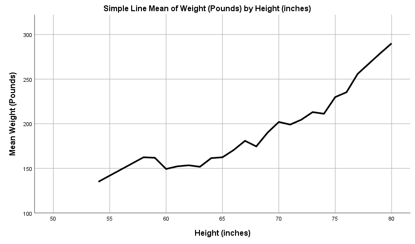
Linear Relationships of Height and Weight
Source: Aoife King (2020)
The above table indicates that there is a linear relationship between the weight of an individual and their height. The relation is seen to be positive as the line is upwards, which means an increase in height brings about a corresponding increase in weight.
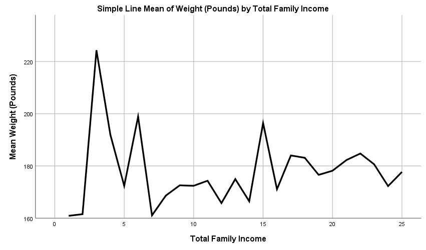
Linear Relationships of Weight and Income
Source: Aoife King (2020)
The above table indicates no linear relationship between total family income and weight. It can be seen in the above graph that there are many fluctuations in the data which means that there is no linear pattern.
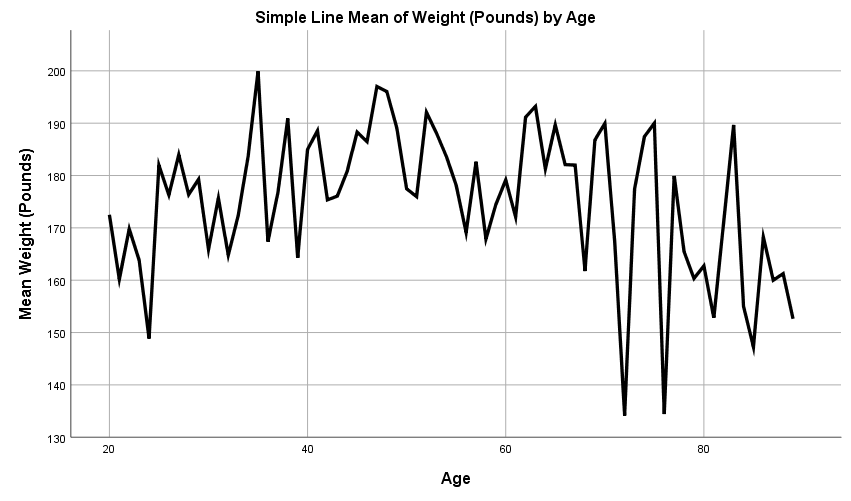
Linear Relationships of Age and Weight
Source: Aoife King (2020)
The above table indicates that there is no linear relationship between the age of an individual and their weight. It can be seen in the above graph that there are many fluctuations in the data which means that there is no linear pattern.
Descriptive Statistics

Descriptive Statistics
Source: Aoife King (2020)
The above table shows the statistical characteristics of the variables GSS considered. Mean is regarded as one of the most widely accepted measures of central tendency. The average age among the 1351 respondents is 16.6 years, meaning that most of the respondents were young adults. The data of age is fairly symmetrical, given the value of 0.21 for skewness. The kurtosis value for this variable is -0.77, meaning that the dataset is light-tailed and called party-kurtas. The average family income among the 1351 respondents is $35000 to $ 39999. The data on family income is highly skewed, given the value of -0.722 for skewness. The kurtosis value for this variable is 0.37, meaning that the dataset is heavy-tailed and called lepto-kurtic. The average height among the 1351 respondents is 66.93 inches. The data of height is fairly symmetrical, given the value of 0.189 for skewness. The value of kurtosis for this variable is -0.560, which means that the dataset is light-tailed and called party-kurtas. The average weight among the 1351 respondents is 178.19 pounds. The data of weight is highly skewed, given the value of 1.11 for skewness. The value of kurtosis for this variable is 4.068, which means that the dataset is heavy-tailed and called lepto-kurtic. The mean value of smoking status showed that most of the respondents were non-smokers, and the value for gender shows that there was an almost equal number of males and females in the GSS data set.
Multiple Regression
After testing the data for assumptions, multiple regression was applied to the data set to see the influence of independent variables (age, gender, smoking status, height, and family income) on the dependent variable (weight in pounds). The methods and materials section mentioned that the data was analysed using SPSS. Considering the number of independent variables in the model, multiple regression was applied to the data to test the relationship and impact. The following table shows the results obtained from SPSS:
| Regression Analysis | ||||||
| Intercept | Age | Gender | Smoking Status | Height | Family Income | |
| Beta Value | -127.123 | -0.38 | -8.590 | 11.195 | 4.663 | -0.504 |
| Standard Error | 25.755 | 0.064 | 2.935 | 2.575 | 0.361 | 0.199 |
| T-stat | -4.936 | -0.597 | -2.927 | 4.347 | 12.902 | -2.541 |
| P-value | 0.000 | 0.551 | 0.003 | 0.000 | 0.000 | 0.011 |
| F-statistic | 90.729 | |||||
| Sig. Value | 0.000 | |||||
| R-squared | 0.252 | |||||
| Adjusted R-squared | 0.249 | |||||
Ordinary Least Squares
Source: Aoife King (2020)
The above table shows all the relevant information required to analyse the significance and extent of the association/relationship of the different predictor variables with the dependent variable, a person’s weight. The table's top portion indicates the coefficient values and their respective sig values and shows whether or not there is statistical relevance in their relationship.
The first predictor variable, Age, was tested against the weight in pounds of the respondents. The p-value assigned to this variable is 0.551, which lies outside the benchmark of 0.05 or below; thus, the individual impact of age on the weight of individuals is found to be statistically insignificant. As the relationship is insignificant, the beta value is irrelevant since it depicts the extent of change in the weight caused by one unit change in age. Nevertheless, these figures highlight a successful Statistical analysis of healthcare data targeted in this study.
Second, the impact of gender is tested on an individual's weight, whether being a specific gender influences a person's weight. The p-value assigned to this variable is 0.003, which lies within the benchmark of 0.05 or below. Thus, the personal impact of gender on the weight of individuals can be said to be statistically relevant and significant. The beta value for this variable shows a negative sign which means that females have a lower weight which is also supported by previous literature. The beta value is 0.859, which means that compared to males, the weight of females is 0.859 pounds less. The following graph visualizes this data:
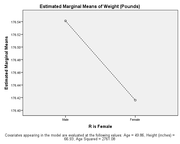
Graph of Gender and Weight
Source: Aoife King (2020)
The next variable to be tested was smoking status, whether or not an individual smokes. The p-value assigned to this variable is 0.000, which lies within the benchmark of 0.05 or below. Thus, the individual impact of an individual being a smoker on the weight of that individual can be said to be statistically relevant and significant. The beta value for this variable is 11.195, meaning that the individuals who do not smoke have 11.195 pounds higher weight than those who do not smoke. The following graph can better understand this:
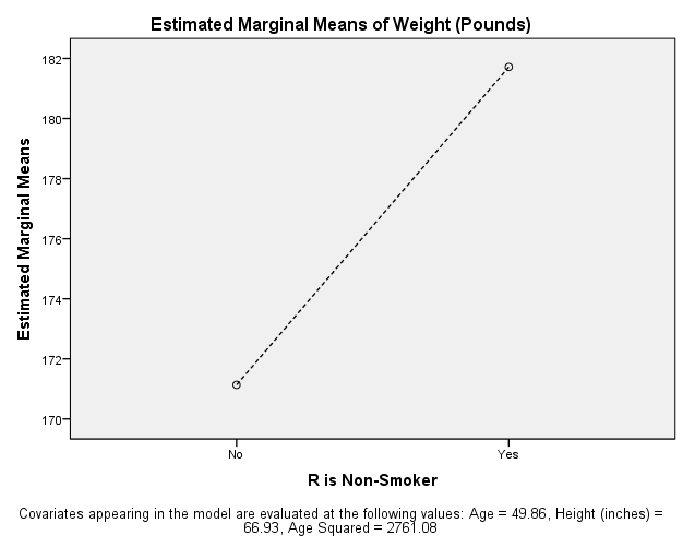
Graph of Smoking Status and Weight
Source: Aoife King (2020)
The next individual attribute that was tested was height in inches; whether being taller or shorter impacts a person’s weight or not. The p-value assigned to this variable is 0.000, which lies within the benchmark of 0.05 or below. Thus, the individual impact of an individual’s height on their weight can be said to be statistically relevant and significant. The beta value for this variable is 4.663, which indicates that if an inch of height of an individual is increased, it will bring about 4.663 units of change in a person's weight.
The last variable obtained through the Statistical data analysis of healthcare data is total family income which is not a personal attribute but a social factor. The impact of this variable was also tested on an individual's weight, whether belonging to a certain income group impacts a person’s weight or not. The p-value assigned to this variable is 0.011, which lies within the benchmark of 0.05 or below. Thus, the individual impact of total family income on the weight of individuals can also be said to be statistically relevant and significant. The beta value for this variable is -0.504, which indicates that higher family income is associated with lower weight considering that a negative sign is associated with it.
In the table's bottom section, certain values explain the entire model, including all the predicting factors and criterion variables. Sig. values determined the complete statistical relevance of the model. The p-value assigned to the model is 0.000, which lies within the benchmark of 0.05 or below. Thus, the overall and collective impact of total family income, age, gender, height, and smoking on the weight of individuals is found to be statistically relevant and significant. R-squared is an important value to be interpreted when explaining ordinary least squares regression in a detailed manner. R-squared, also known as the coefficient of determination, is the proportion of the variance in the dependent variable that is predictable from the independent variables. In the case of the model being considered here, total family income, age, gender, height, and smoking can explain 0.252 or 25.2% of respondents' weight variation. Lastly, an adjusted R-square can be referred to as a modified version of the coefficient of determination which is adjusted by the number of independent variables in the model. Thus, after adjustment, total family income, age, gender, height, and smoking can explain 0.249 or 24.9% of individuals' weight variation.
The following text comprises the discussion of the study.
Discussion
There is abundant research on the impact of different personal and social attributes and their influence on a person’s weight. This study was focused on finding the age associations with weight through Statistical analysis of healthcare data including physical and social attributes. In this study, a direct relationship between age and weight was not evaluated; rather, the author aimed to study how age influences weight. The research results showed that age significantly correlates with obesity among men and women aged 30-74, which was the sample size. However, from the primary findings, it can be evaluated that there is no significant individualistic impact of age on weight.
Research conducted by Lopez et al. (2018) to analyse the influence of gender on obesity found in the study has indicated that females are more prone to be obese than women. However, it is important to consider that this study evaluated rats as their sample. This means that there can be differences in the results of this research. From this research, it has been found that women tend to weigh lighter than men. The primary results of this research showed a positive impact of income and height on the weight of individuals. It is commonly accepted that a person with a greater height will also have more weight because of their bones. The study by Buser et al. (2016) aimed to assess the impact of changes in income on the height and weight of young children. The sample for this research comprised young children of families in Ecuador. The results of this research indicated no significant influence of changes in income on the heights and weights of young children. This research showed that higher income is inversely related to an individual's weight. It is important to consider that when the linearity of the relationship of income was tested against weight, it was found that a linear relationship did not exist among them. This research has also concluded that people who smoke tend to weigh lighter as compared to individuals who are non-smokers. This stance can also be supported by previous literature (Berlin et al., 2017).
The results have indicated that the model is relevant in statistical terms as the overall sig value is less than the benchmark value of alpha. However, while judging the attributes individually, it was found that age does not tend to impact an individual's weight.
Conclusion
The overall model was significant, and a substantial impact of the independent variables over the dependent variable was found. However, when the impact of the variables was checked individually, the relationship between age and weight was found to be insignificant. While conducting the study, two assumptions were made regarding the data; that the data is normally distributed and that there is no multicollinearity among the variables. However, while the assumption regarding the multicollinearity was correct, the data was not found to be normally distributed. The result of testing has further shown that there is a linear relationship between height and body weight, which means that if the height of a person increases, there is a greater probability that the person's weight would also increase, which is to be expected. Lastly, the relationship between weight and income was also tested, along with the relation between age and weight. It was observed that there is a non-linear relationship between the variables respectively.
References
Atalay, S.D., Calis, G., Kus, G. and Kuru, M., 2019. Performance analyses of statistical approaches for modelling electricity consumption of a commercial building in France. Energy and Buildings, 195, pp.82-92.
Berlin, I., Golmard, J.L., Jacob, N., Tanguy, M.L. and Heishman, S.J., 2017. Cigarette smoking during pregnancy: do complete abstinence and low-level cigarette smoking have a similar impact on birth weight? Nicotine & Tobacco Research, 19(5), pp.518-524.
Bowman, K., Delgado, J., Henley, W.E., Masoli, J.A., Kos, K., Brayne, C., Thokala, P., Lafortune, L., Kuchel, G.A., Ble, A. and Melzer, D., 2016. Obesity in older people with and without conditions associated with weight loss: follow-up of 955,000 primary care patients. Journals of Gerontology Series A: Biomedical Sciences and Medical Sciences, 72(2), pp.203-209.
Buser, T., Oosterbeek, H., Plug, E., Ponce, J. and Rosero, J., 2016. The impact of positive and negative income changes on the height and weight of young children. The World Bank Economic Review, 31(3), pp.786-808.
Converse, J.M., 2017. Survey research in the United States: Roots and emergence 1890-1960. Routledge.
Etikan, I. and Bala, K., 2017. Sampling and sampling methods. Biometrics & Biostatistics International Journal, 5(6), p.00149.
Etikan, I. and Bala, K., 2017. Sampling and sampling methods. Biometrics & Biostatistics International Journal, 5(6), p.00149.
Jebb, A.T., Parrigon, S. and Woo, S.E., 2017. Exploratory data analysis as a foundation of inductive research. Human Resource Management Review, 27(2), pp.265-276.
Koo, T.K. and Li, M.Y., 2016. A guideline for selecting and reporting intraclass correlation coefficients for reliability research. Journal of Chiropractic Medicine, 15(2), pp.155-163.
Lavie, C.J., Arena, R. and Blair, S.N., 2016. A call to increase physical activity across the globe in the 21st century.
López, N., Sánchez, J., Palou, A. and Serra, F., 2018. Gender-associated impact of early leucine supplementation on adult predisposition to obesity in rats. Nutrients, 10(1), p.76.
Myers, A., Gibbons, C., Finlayson, G. and Blundell, J., 2017. Associations among sedentary and active behaviours, body fat and appetite dysregulation: investigating the myth of physical inactivity and obesity. Br J Sports Med, 51(21), pp.1540-1544.
Padley, M. and Marshall, L., 2018. Defining and measuring housing affordability using the Minimum Income Standard Housing Studies. Housing Studies, pp.1-23.
Pietilä, A.M., Nurmi, S.M., Halkoaho, A. and Kyngäs, H., 2020. Qualitative Research: Ethical Considerations. In The Application of Content Analysis in Nursing Science Research (pp. 49-69). Springer, Cham.
Stevens, J., 2000. Impact of age on associations between weight and mortality. Nutrition Reviews, 58(5), pp.129-137.
Taherdoost, H., 2016. Validity and reliability of the research instrument; how to test the validation of a questionnaire/survey in
 Download PDF File
Get 3+ Free Dissertation Topics within 24 hours?


