


Applied Corporate Strategy
July 9, 2022
Case of Tesla Merger with Solar City
July 9, 2022
In delving into Portfolio Review and Remedial Options Actions, this study conducts a comprehensive analysis, unravelling the intricacies of optimizing investment portfolios and presenting strategic pathways for remedial actions beyond conventional approaches.
In the world of investments, maintaining a healthy and productive portfolio is paramount. Whether you are an individual investor or a financial professional, regularly reviewing your portfolio is essential. It is through these reviews that you can gauge how well your investments are performing and make informed decisions to meet your financial goals.
Explore More About Portfolio Review
In this blog, we'll delve into the importance of portfolio reviews and explore various remedial options and actions to optimize your investments. These actions can help you manage risks, align your portfolio with changing financial goals, and enhance tax efficiency. By staying vigilant and adaptable, you can navigate the ever-changing landscape of financial markets and work toward achieving your financial goals.


Introduction
This study encompasses several key elements. Firstly, it begins by thoroughly examining Miss I. Ohri's Investment Policy Statement, shedding light on the objectives of her investment strategy and her future financial plans. Secondly, it constructs a diversified portfolio utilizing UK FTSE 100 stocks and UK Government Bonds. This entails a comprehensive analysis of the potential benefits of investing in a subset of 30 FTSE stocks through correlation analysis, drawing from the insights of Barberis, Mukherjee, and Wang (2016).
To facilitate this analysis, historical data on share prices for UK FTSE 100 stocks spanning the past 11 years will be collected and assessed. The study will also delve into Covariance, Correlation, Regression, and Descriptive Statistics, applying data analysis techniques to evaluate the performance of this diverse 100-stock portfolio. Special attention will be given to analyzing the returns and excess returns associated with these securities, focusing on selecting the most promising 30 stocks from the FTSE 100 index.
The third component of this study involves demonstrating how to determine the Optimum Risky assets using the Markowitz Portfolio Optimization Model and the Traynor-Black Model. Subsequently, it will evaluate the portfolio's performance over 10 years. Finally, the study will provide an in-depth analysis of the portfolio's performance in the most recent year, drawing from insights shared by Lasher in 2013.
Investment Policy Statement
What is an “Investment Policy Statement” – IPS?
An Investment Policy Statement (IPS) serves as a formal document that outlines a comprehensive agreement between a portfolio manager and a client. This document succinctly encapsulates the overarching investment strategies to be employed by the manager. Within the IPS, the client's investment goals and objectives are precisely articulated, and the tactics the manager intends to employ to pursue these objectives are defined. Notably, the IPS contains essential information regarding critical aspects such as asset allocation, risk tolerance, and liquidity requirements, which are integral to the investment strategy. (Source: Investopedia, 2017).
As an illustrative example, an Investment Policy Statement can be presented in the following manner:
Investment Policy Statement (IPS)
Client name: Iva Ohri
Status: (Single)
Age: 35
Retirement age: 65 years old
Address: 9 Stevenage Road, East Ham, London
Postal Code: E62AU
e-mail: i
………………………………………………………………………………………………………………………………………
Investor Conditions
Due to the investor’s actual studies in MSc in Global Investments and Finance in London, she isn’t interested in buying a new house. Still, she is interested in investing in other stocks, and the money saved should be managed consequently for 5 years (Andersen & Glenn,2014).
The Investor defines their understanding of investments as limited.
The predictable position for the Investors’ economic condition:
Modesty adverse over the next year (because of her studies);
Modesty optimistic over the next five years;
Very positive over the next ten years.
Iva Ohri is currently living in London, following her studies. She is paying a monthly rent of £500. Her monthly expenses are approximately £850. In addition to the money she saved (approximately £7000), she owns another savings account in Albania.
…………………………………………………………………………………………………………………………………………
Overview
The following facts are a summary of the Investor outline, created based on the evidence that she provided:
Twelve-monthly family income (before tax) is £10,000 to £15,000;
Possibly will tolerate a provisional decline in her portfolio over one year of -4%;
She has some investment knowledge;
Her existing investment portfolio embraces equal amounts of fixed profits and securities.
Investment Aims/Objectives
The Investor’s principal objective for the investment portfolio is to produce profits from investing in properties in London and to achieve growth.
Investor’s Risk Tolerance: Traditional
Investment Time Horizon
She has acknowledged her portfolio’s investment time horizon to be 10 – 20 years.
Methodology
The research methodology employed in this study will encompass descriptive statistics and a critical analysis of calculations carried out using an Excel Sheet. This Excel Sheet will be instrumental in computing the Optimum Portfolio of risky assets for UK FTSE 100 stocks, aligning with principles outlined by Bodie and colleagues in 2014.
To assess the performance of the FTSE 100 stock portfolio, a structured approach will be employed. The first step involves downloading historical data for UK FTSE 100 stocks over the past 11 years and transferring this data into an Excel Sheet. Subsequently, the study will proceed to calculate various metrics, including portfolio returns over the 11 years, the standard deviation of the portfolio, expected returns, annual rates for each stock in the portfolio, the variance-covariance matrix, annual variance, annual standard deviation, weighted portfolio values, and ultimately, the composition of the optimal risky portfolio.
To provide a clearer understanding of this methodology, the following section will present a step-by-step breakdown of the calculations conducted within the Excel Sheet, offering a comprehensive insight into the processes involved in determining the Optimum Portfolio.
Step 1:
Our Benchmark will divide the last year's performance (2016) and then the ten-year performance; it will be shown together in the table. It will be calculated the holding period returns of 100 stocks, using the formula in Excel: So, we will convert the prices into returns using the formula:
Rt = LN (Pt/Pt-1);
In the Excel Sheet, the formula must be: =LN(price today/price yesterday) and then auto-fill the column. For UK Gilt, for example, the formula that will be used is =((1+(Data!B3/100))^(1/12))-1 because we want to exclude UK Gilt when constructing our portfolio. For FTSE 100, the formula for calculating the returns over the 10 years is: =LN(Data!C3/Data!C4)
Step 2:
How do we find the covariance and variance for 100 stocks?
It will be found running Data – Data Analysis – Selecting Covariance and then selecting all the data with the returns for 100 stocks and then running okay. The same thing we will do for finding the Variance of 100 stocks ‘returns Portfolio, running Data – Data Analysis -Selecting Variance, and then selecting all the Returns data of 100 stocks and then pressing ok. Correlation means how all the 100 stocks’ returns occur simultaneously. We also need to find the regression of our portfolio running Data – Data Analysis – Regression – select all the Returns data of 100 stocks and press ok.
Step 3:
We have to choose 30 stocks based on the correlation and alpha. To create an Active Portfolio, the correlation has to be lower enough. Below will be shown the 30 stocks based on the lowest correlations:
(30 Stocks Portfolio)
Ashtead Group |
RBS |
Aviva |
Barrat Developments |
GSK |
British American Tabacco |
LAMB |
ITV |
Persimmon |
Taylor Wimpey |
Wolseley |
Randgold |
HMSO |
TAG |
British Land |
Carnival Corporation & plc |
Easyjet |
BT Group |
Informa |
3i |
London Stock Exchange Group PLC |
Marks & Spenser Group PLC |
Sage Group |
Travis Perkins |
RELAX |
Old Mutual |
KGF |
DCC |
Intu |
Legal & General Group PLC |
Step 4:
After choosing the 30 Stocks Portfolio, it will be demonstrated how to calculate the Optimum Portfolio risky assets using Excel. It will be shown the Portfolio Optimization of 30 Stocks portfolio using the Markowitz Portfolio Optimization Model. This Portfolio theory explains how each of the 30 stocks in a portfolio relates to each other, and it tries to reduce the risk while optimizing returns. What is important to consider in this Model is that we will look for the Optimal Portfolio, which will give us the best risk-return trade-off and that will lie along this minimum variance frontier within a given of risky assets.
In the Excel Sheet, we will look at 30 different stocks that we have already chosen, and we will combine those in the best weights to give us that risk-return trade-off that produces the optimal outcome. So, the Expected Return for a portfolio is calculated as the weights of the assets within the portfolio multiplied by their Expected Return (Portfolio Optimization Youtube, 2017):
E(rp) = ∑ W1 E (ri)
The variance of two assets (X and Y) portfolio is calculated as: (the weight of “X” squared, multiplied by the variance of X squared, plus the weight of “Y” squared multiplied by the variance of Y, plus two times the weight of “X” multiplied by the weight of “Y”, multiplied by the covariance of X and Y or how they move together. So, if we generalize this formula to more than 2 assets, we can use the following equation: the sum of the weights multiplied together for each asset “I” and “j” multiplied by the covariance. The Expected Return for the Portfolio is calculated using matrix notation, where we have the weights of the assets of
our Portfolio transposed multiplied by their expected return, where W – is the vector of weights of the individual assets (i through j) in the Portfolio and R – is the vector of expected returns on the individual assets (i though j) in the portfolio. The Formula in Excel that will be used is:
{=mmult(transpose(W),R)}
Where W – is the Column of Weights and R- is the Column of Expected Returns. When making calculations with arrays in Excel, type in the formula, but don’t press Enter. Instead, we have to hold down [Ctrl] [Shift] and then press [Enter]. This will tell Excel that we are making calculations with an array and put the curly parentheses around the formula.
The Variance of the Portfolio is calculated as the weights of each asset in the Portfolio transposed multiplied by S, where “S” is the variance/covariance matrix and then multiplied again by the weights of the assets in the Portfolio.
The Standard Deviation of the Portfolio will be calculated as the square root of the variance of the Portfolio. The Standard Deviation of the returns of the Portfolio is calculated in Excel as follows:
{=sqrt(multi(multi(transpose(W), S), W))) and then Press [CTRL, SHIFT together and then press [Enter]]
The Optimal weights of the 30 Stocks in our Portfolio are the ones that maximize the value of the sharp ratio for the Portfolio, and it will be shown using “Solver” in Excel to do this.
The optimal mix of weights for the assets in our risky portfolio is the mix that creates a portfolio along the efficient frontier that is tangent with the capital allocation. This results in the capital allocation with the largest slope (sharp ratio) and is, therefore, the optimal risky portfolio.
We are going to choose the stocks that have the higher Sharp ratio and the Risk-free rate we will assume will be 1,07.
The Complete Portfolio | |||
Risky portfolio | Gilt | Complete Portfolio | |
Expected return | 12.00% | 1.07% | 16.62% |
St.Dev | 14.52% | 0 | 20.66% |
A | 4 | Sharpe | |
Optimal weight: | 142.27% | -42.27% | 0.7527 |
Our Sharp ratio will be calculated in Excel as =(Expected Return – Risk-free rate)/Standard Deviation of the Portfolio.
So, the highest Sharp ratio in our 30 Stocks Portfolio is 0,752. And our Expected Return Portfolio is 12% with a Standard Deviation of 14 52%.
Our Optimal Weight in our Risky Portfolio is 142.27% with a risk aversion of 4.
Also, if we look at our Complete Portfolio, our Expected Return is 16.62% with a Standard Deviation of 20, 66% (the measure of risk in our Portfolio), and an Optimal weight of 0.7527.
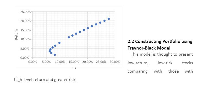
The portfolio is found in the Graph below. The golden rule of an investor is that an Investor can take more risk investing in these 30 stocks only if they can achieve that higher level of return. Similarly, Investors can get a higher level of return if they are willing to take that extra risk (Mangram, 2013). No investor should invest below the 5% expected return because it will increase the returns while decreasing risk (Markowitz, 2014). So, the Graph shows that the lower the risk in a portfolio, the higher the return. Investors should be interested in an efficient portfolio, which means a portfolio where the relationship between risk and return is such that we can get a higher return only by taking a little extra risk. The Investor should be interested in taking all this extra risk because it should bring a higher return (Markowitz, 2014). One thing that we want to know is where the inefficient frontier end and the efficient portfolio start to do. Well, it will be the point on the graph below, where the Standard Deviation is the lowest (it will be the lowest risky portfolio), and we call this the Minimum Variance Portfolio (Mangram, 2013).


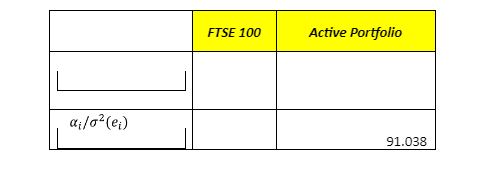
Constructing Portfolio Using Traynor-Black Model
Constructing a portfolio using the Traynor-Black Model is a strategic endeavour that aims to optimize the allocation of assets within an investment portfolio. This model, developed by Jack Treynor and Fischer Black, places a strong emphasis on assessing and balancing the systematic and unsystematic risks associated with various assets. By determining the ideal mixture of passively and actively managed stocks, investors can work to achieve a more efficient and balanced portfolio, ultimately seeking to strike the right balance between risk and return.
Advantages and Disadvantages of Using the Markowitz Optimization Model & Traynor-Black Model
The advantages of incorporating portfolio planning with the efficient frontier, often harnessed through the "Markowitz Optimization Model," become evident when evaluating the relationship between risk and return. The efficient frontier, graphically represented as an arched line, juxtaposes the expected portfolio return on the "y" axis against the portfolio's standard deviation or risk on the "x" axis. This model, attributed to the renowned Harry Markowitz, often hailed as the "father of portfolio management" (Wallengren & Sigurdson, 2017), forms the basis of Modern Portfolio Theory.
This theory is a comprehensive approach to portfolio investment, encompassing a thorough examination of the broader market and the economy. It endeavours to elucidate how each stock within a portfolio interrelates with others, all while striving to minimize risk while maximizing returns. The Modern Portfolio Theory accounts for the returns of assets along with their systematic and unsystematic risk, as aptly noted by Mangram in 2013. By considering both return and risk in the context of a portfolio, it constructs a line that delineates all available portfolio options, commonly referred to as the efficient frontier. To attain optimal risk-return ratios, a portfolio should ideally gravitate toward or closely align with this efficient frontier. Portfolios falling below this threshold typically entail an excessive amount of risk for the expected return, as described by Investopedia (2017).
The "Treynor-Black Model," conceived by Jack Treynor and Fischer Black, is an asset allocation model designed to determine the optimal blend of passively and actively managed stocks within an investment portfolio. Once the optimal allocation of stocks is established, the model predominantly focuses on the systematic and unsystematic risk associated with these stocks, as outlined by Gerber, Markowitz, and Pujara in 2015.
Nevertheless, the drawback of the Treynor-Black Model lies in its relatively limited emphasis on the "Beta" of stocks and their unsystematic risk. Stocks with higher unsystematic risk are given less weight in this model, potentially leading to a portfolio comprising low-return, low-risk stocks when compared to those offering higher returns and greater risk, as noted by Investopedia (2017).
Critically Analyse Portfolios’ Risk-Return Profiles
The analysis of a portfolio's risk-return profile hinges on the appropriate model, considering 10-year performance data and abnormal returns from the previous year. The Treynor-Black Model is a comprehensive approach that assesses active investment strategies and asset allocation within the framework of the market portfolio. However, it relies on specific underlying assumptions to remain valid. One such assumption is the active involvement of security analysts in managing the organization, delving deep into a relatively small number of stocks within the vast universe of securities (Brown, 2015).
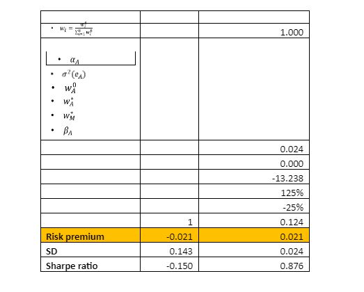
Treynor's measure provides a basis for comparing portfolios, primarily focusing on the alpha-to-beta ratio. In the case of the FTSE security portfolio, the alpha is forecasted as 0, while the risk premium is -0.214, and the standard deviation of the portfolio stock is 0.1425. Conversely, for the optimal risky portfolios, the premium, standard deviation, and Sharpe's ratio values change. These alterations occur in response to shifts in the stock parameters, such as a beta of 1, a risk premium of -0.021, and a standard deviation of 0.143, along with a -0.150 (insert unit) (reference).
Sharpe's approach involves regressing portfolio returns on indices representing a broad spectrum of asset classes. Consequently, the regression coefficient of each index serves as an indicator of the fund's implicit allocation. Given the constraints on these funds, the regression coefficients are typically constrained to be zero or positive, with a total sum of 100 to achieve a full asset allocation (Imai, Van Deventer, & Mesler, 2013). An alpha value of zero implies that deviating from a passive strategy would not add value, and the performance of the index portfolio would predominantly rely on the managers' decision-making. However, it's important to recognize that this scenario is quite rare. Consequently, assessing the impact of one security purchase over another necessitates the utilization of Markowitz models, which consider risk and return factors and employ portfolio diversification to mitigate the impact of risk through diversification (Yang & Yeh, 2015).
Review Portfolio Performances
Evaluating portfolio performance and implementing effective rebalancing as part of remedial actions involves the practical application of the Markowitz model. This model empowers investors to make informed decisions about the trade-off between risks and returns, spanning from minimal to potentially infinite levels of risk. In the context of a 100FTSE stock portfolio, this trade-off is particularly evident (Guerard, 2016). Calculating the mean return for the portfolio stock is a crucial step, which can be determined using the respective portfolio weights (refer to the FTSE 100 calculation).
Utilizing the attached values, the computation of expected portfolio returns involves the application of these weights. For example, if we have weights (wa, wb, etc.) and corresponding returns (Ba, Bb, etc.), the expected portfolio return can be calculated as follows: Expected Return = wa * Ba + wb * Bb + ... + wn * Bn. In practice, this can be demonstrated as follows: Expected Return = 125% * 0.124 + (-25%) * 0.024 = 0.155 - 0.006 = 0.149.
Assessing the risky nature of the portfolio entails closely examining its beta, a measure of its risk about the broader market. The implication of this beta value is critical for investors in gauging the overall risk of the portfolio. The optimal combination of an active portfolio with a passive one stems from creating an optimal risky portfolio, often composed of two risky assets. This construction involves applying Sharpe's ratio, as articulated by Brigham and Ehrhardt (2013).
In this context, the active portfolio perfectly correlates with the index, indicating the need for diversification. Mixing the active portfolio with the index can potentially yield higher returns and is a strategy often pursued by investors. The success of active management, the contribution of the active portfolio as measured by the Sharpe ratio, and the risky portfolio are compared to the index portfolio (Brown, 2015). Consequently, in assessing the FTSE 100 portfolio stock, it becomes evident that diversification remains the primary available strategy to mitigate the impact of market risk in this scenario.
Analysis of the 30 Stocks Portfolio (2016)
The performance of the stock portfolio, in connection with the FTSE market index, unveils important insights. Notably, the portfolio's beta values range from 0.1 to 0.8, indicating varying levels of risk within the individual portfolio components. However, these values tend to decrease when the portfolio is diversified, a trend evident in the portfolio's standard deviation combinations.
When assessing the individual stocks within the portfolio based on their alpha, beta, risk premium, and standard deviation parameters, an interesting pattern emerges. Approximately 10 % of the stocks display lower levels of risk, while roughly 40 % fall into the category of being moderately risky. In contrast, a significant portion, approximately 50 %, of the stocks are categorized as highly risky. This distribution underscores the importance of diversification as a critical strategy for mitigating the impact of these risks and achieving a more balanced and stable portfolio.
Conclusion
References
Andersen, K., & Glenn, P. (2014). Portfolio Preservation During Severe Market Corrections: A Market Timing Enhancement to Modern Portfolio Theory.
Barberis, N., Mukherjee, A., & Wang, B. (2016). Prospect theory and stock returns: an empirical test. The Review of Financial Studies, 29(11), 3068-3107.
Bodie, Z., Kane, A., & Marcus, A. J. (2014). Investments, 10e. McGraw-Hill Education.
Brigham, E. F., & Ehrhardt, M. C. (2013). Financial management: Theory & practice. Cengage Learning.
Brown, A. D. (2015). The Power of an Actively Managed Portfolio: an Empirical Example Using the Treynor-Black Model (Doctoral dissertation, The University of Mississippi).
Dhrymes, P. J. (2017). Portfolio Theory: Origins, Markowitz and CAPM Based Selection. In Portfolio Construction, Measurement, and Efficiency (pp. 39-48). Springer International Publishing
FTSE 100 Index, 2017. The online UK Stock Exchange Review. Available online at: www.ftse100.co.uk [Retrieved 12 August, 2017]
Gerber, S., Markowitz, H., & Pujara, P. (2015). Enhancing Multi-Asset Portfolio Construction Under Modern Portfolio Theory with a Robust Co-Movement Measure.
Google Images, 2017. Image extracted from: Google/ipwatchdog.com [Retrieved 12 August, 2017]
Guerard Jr, J. B. (Ed.). (2016). Portfolio Construction, Measurement, and Efficiency: Essays in Honor of Jack Treynor. Springer.
Imai, K., Van Deventer, D. R., & Mesler, M. (2013). Advanced financial risk management: tools and techniques for integrated credit risk and Interest rate management.
Investment Policy Statement, 2017. Available online at: www.investopedia.com/terms/i/ips.asp [Retrieved 15 August 2017]
Lasher, W. R. (2013). Practical financial management. Nelson Education.
Mangram, M. E. (2013). A simplified perspective of the Markowitz portfolio theory.
Markowitz, H. (2014). Mean-variance approximations to expected utility. European Journal of Operational Research, 234(2), 346-355.
Yang, S. S., & Yeh, Y. Y. (2015). Analysis of the Efficient Frontier for Life Settlements in the Presence of Longevity Risk. 財務金融學刊, 23(1), 1-29.
Wallengren, E., & Sigurdson, R. S. (2017). Markowitz portfolio theory.
Get 3+ Free Dissertation Topics within 24 hours?